Twiss
Xtrack provides a twiss method associated to the line that can be used to
obtain the twiss parameters and other quantities like tunes, chromaticities,
slip factor, etc. This is illustrated in the following example. For a complete
description of all available options and output quantities, please refer to the
xtrack.Line.twiss() method documentation.
Basic usage
import numpy as np

import xtrack as xt
import xpart as xp

#################################
# Load a line and build tracker #
#################################

line = xt.Line.from_json(
    '../../test_data/hllhc15_noerrors_nobb/line_and_particle.json')
line.particle_ref = xp.Particles(
                    mass0=xp.PROTON_MASS_EV, q0=1, energy0=7e12)
line.build_tracker()

#########
# Twiss #
#########

tw = line.twiss()
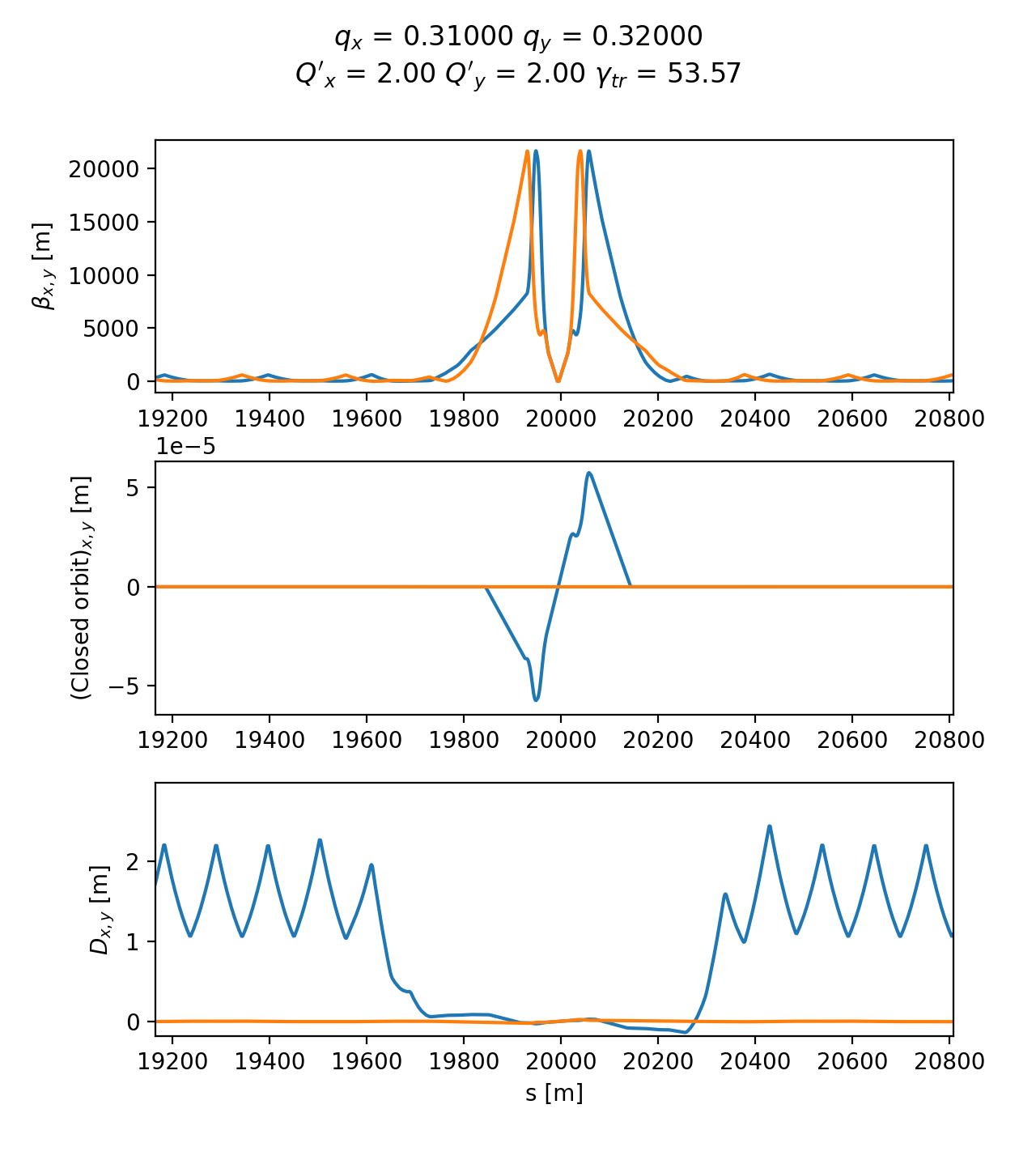
Twiss functions and accelerator parameters as obtained by Xtrack twiss. See the full code generating the image.
Access option of twiss table
The twiss table has several access options as illustrated in the following example.
import numpy as np

import xtrack as xt
import xpart as xp

# Load a line and build tracker
line = xt.Line.from_json(
    '../../test_data/hllhc15_noerrors_nobb/line_and_particle.json')
line.particle_ref = xp.Particles(
                    mass0=xp.PROTON_MASS_EV, q0=1, energy0=7e12)
line.build_tracker()

# Twiss
tw = line.twiss()

# Examples of access modes to the twiss table

tw['qx']
# gives : 62.3100009

tw.qx
# gives : 62.3100009

tw['betx']
# gives a numpy array with the beta horizontal beta function along the line

tw.betx
# give the same as above

tw[:, 'ip1']
# gives a table with all the columns at the element `ip1`

tw[:, ['ip1', 'ip2']]
# gives a table with all the columns at the elements `ip1` and `ip2`

tw['betx', 0]
# gives the beta horizontal beta function at the first element

tw['betx', 'ip1']
# gives the beta horizontal beta function at the element `ip1`

tw[:, 'ip.*']
# gives a table with all the columns at all elements whose name matches the

tw['betx', 0:10]
# gives the horizontal beta function at the first 10 elements

tw['betx', 'ip1': 'ip2']
# gives the horizontal beta function at all elements between `ip1` and
# `ip2`

tw[['s', 'betx', 'bety'], 'ip.*']
# returns a table with the horizontal and vertical beta function at all
# elements whose name matches the regular expression `ip.*`

tw[['s', 'betx', 'bety'], 200:300:'s']
# returns the selected columns all the elements between s=200 and s=300

tw[:, 'ip1%%-5': 'ip1%%+5']
# returns a table with all the columns at elements located between 5 elements
# before and 5 elements after the element `ip1

tw[['betx','sqrt(betx)/2/bety'], 'ip1': 'ip2']
# returns a table including the required columns

tw.cols['betx']
# returns a table with the horizontal beta function along the line

tw.cols['betx', 'sqrt(betx)/2/bety']
# returns a table with the horizontal beta function and specified computation

tw.rows['ip1':'ip2', 'mcb.*']
# returns a table with the columns matching the regular expression `mcb.*`
# at all elements between `ip1` and `ip2`

tw.rows['ip1':'ip2', 'mcb.*'].cols['betx', 'sqrt(betx)/2/bety']
# returns a table with the horizontal beta function and specified computation
# at all elements between `ip1` and `ip2` matching the regular expression
4d method for twiss and build_particles
When the RF cavities are disabled or not included in the lattice or when the longitudinal motion is artificially frozen, the one-turn matrix of the line is singular, and it is no possible to use the standard method for the twiss calculation and to generate particles distributions matched to the lattice. In these cases, the “4d” method can be used, as illustrated in the following examples:
import json
import numpy as np

import xobjects as xo
import xtrack as xt
import xpart as xp

#####################################
# Load a line and build the tracker #
#####################################

fname_line_particles = '../../test_data/hllhc15_noerrors_nobb/line_and_particle.json'

with open(fname_line_particles, 'r') as fid:
    input_data = json.load(fid)
line = xt.Line.from_dict(input_data['line'])
line.particle_ref = xp.Particles.from_dict(input_data['particle'])

line.build_tracker()

# We consider a case in which all RF cavities are off
for ee in line.elements:
    if isinstance(ee, xt.Cavity):
        ee.voltage = 0

##################
# Twiss(4d mode) #
##################

# For this configuration, `line.twiss()` gives an exception because the
# longitudinal motion is not stable.
# In this case, the '4d' method of `line.twiss()` can be used to compute the
# twiss parameters.

tw = line.twiss(method='4d')

###########################################
# Match a particle distribution (4d mode) #
###########################################

# The '4d' method can also be used to match a particle distribution:

particles = line.build_particles(method='4d',
                    x_norm=[1,2,3,4], # sigmas
                    nemitt_x=2.5e-6, nemitt_y=2.5e-6)
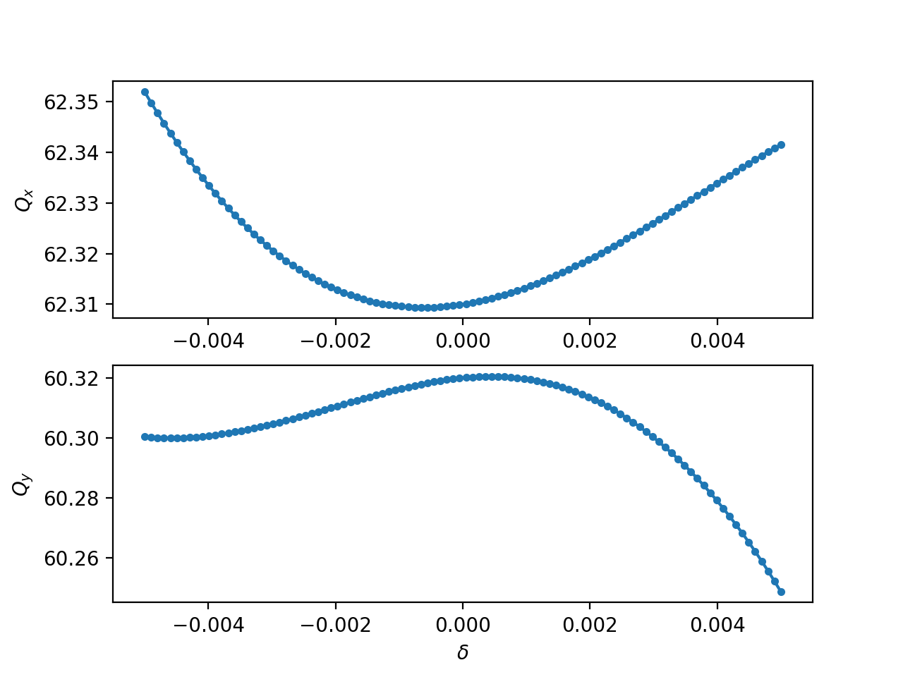
Non linear momentum detuning
The 4d mode of the twiss can be used providing in input the initial momentum. Such a feature can be used to measure the non linear momentum detuning of the accelerator as shown in the following example:
import numpy as np
from cpymad.madx import Madx

import xtrack as xt
import xpart as xp

mad = Madx()
mad.call('../../test_data/hllhc15_noerrors_nobb/sequence.madx')
mad.use('lhcb1')

line = xt.Line.from_madx_sequence(mad.sequence.lhcb1)
line.particle_ref = xp.Particles(p0c=7000e9, mass0=xp.PROTON_MASS_EV)

line.build_tracker()

tw = line.twiss()

delta_values = np.linspace(-5e-3, 5e-3, 100)

qx_values = delta_values * 0
qy_values = delta_values * 0
for i, delta in enumerate(delta_values):
    print(f'Xsuite working on {i} of {len(delta_values)}  ', end='\r', flush=True)
    tt = line.twiss(method='4d', delta0=delta)

    qx_values[i] = tt.qx
    qy_values[i] = tt.qy